Creating A Pie Chart In Excel

In Excel Click on the Insert tab. Then click the Insert tab and click the dropdown menu next to the image of a pie chart. Click the chart and then click the icons next to the chart to add finishing touches.

sizing conversion chart shoes maplestory dps chart 2019 gms 2019 ram 1500 towing capacity chart 21 day fix calorie chart how to use a smith chart eagles stadium seating chart inch to mm conversion chart read through the bible in a year chart

You can select between 2D 3D and Doughnut charts.

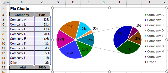
Creating a pie chart in excel. Besides it only takes a couple of clicks to make such charts. Creating Pie of Pie Chart in Excel. From the dropdown menu that appears select the Bar of Pie option under the 2-D Pie category.

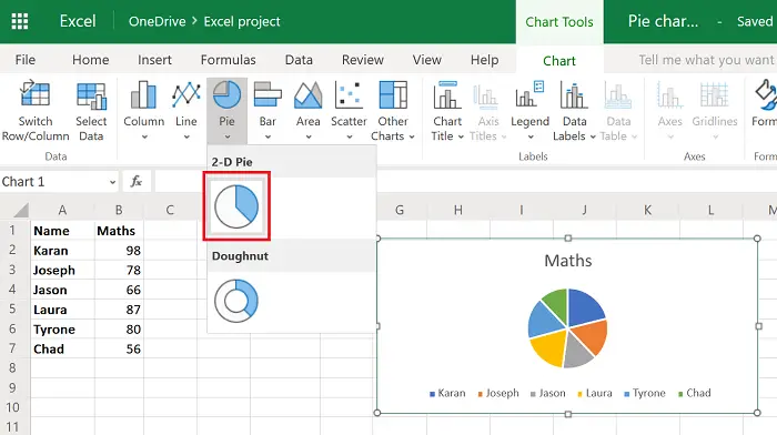
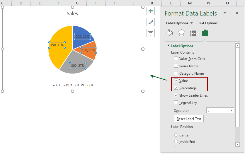
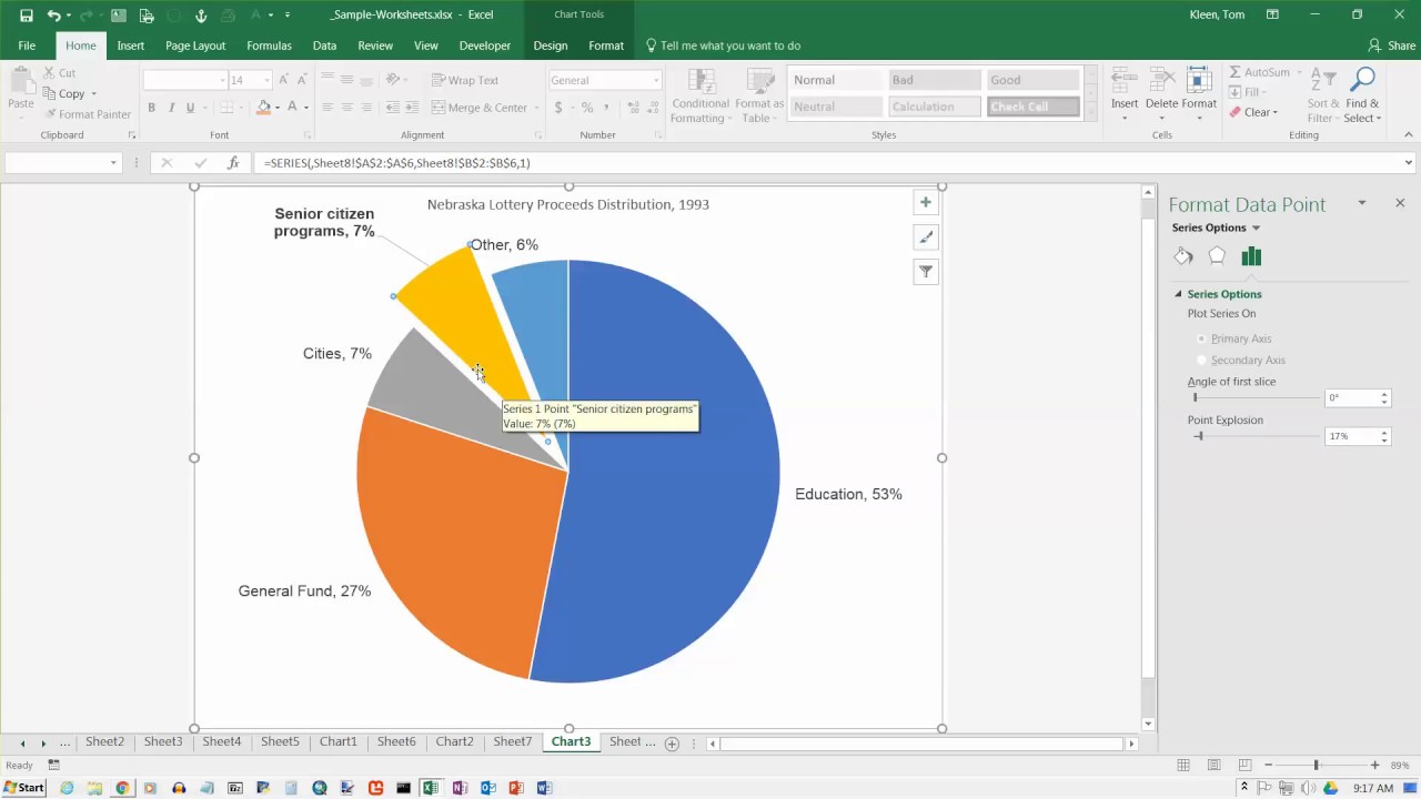
Pie or Doughnut Chart Icon. Select the entire dataset. Then you can add the data labels for the data points of the chart please select the pie chart and right click.

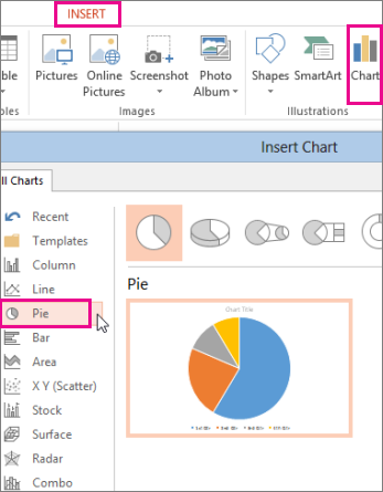
Click Insert Insert Pie or Doughnut Chart and then pick the chart you want. This will add all the values we are showing on the slices of the pie. Select the chart type you want to use and the chosen chart will appear on the worksheet with the data you selected.

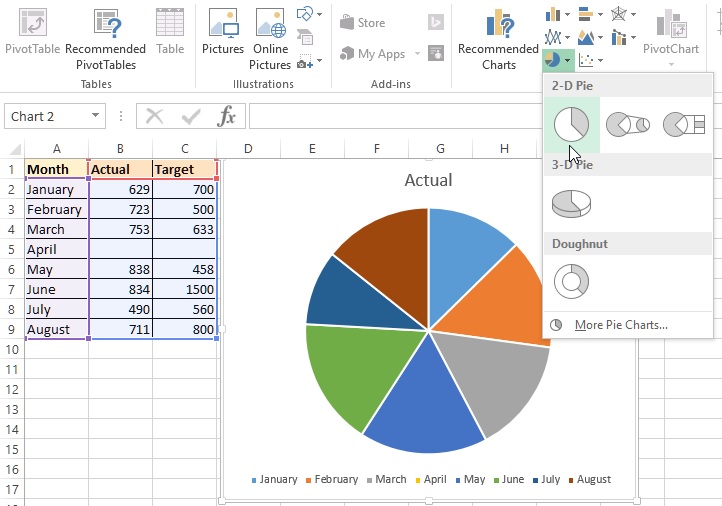
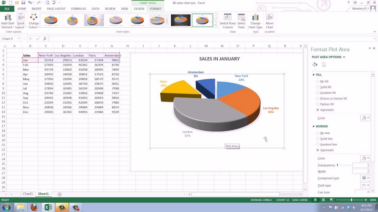
Now it instantly creates the 3-D pie chart for you. Despite there being a wide array of charts that can be created creating Pie charts in Excel is one of the slightly more. Once you have the data in place below are the steps to create a Pie chart in Excel.

How do I make a pie chart in Excel from one column. Right-click on the pie and select Add Data Labels. To create a pie chart in Excel 2016 add your data set to a worksheet and highlight it.

In Excel Click on the Insert tab. Select the chart type you want to use and the chosen chart will appear on the worksheet with the data you selected. Click the Insert tab at the top of the screen then click on the pie chart icon which looks like a pie chart.

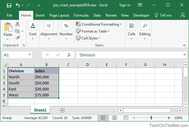
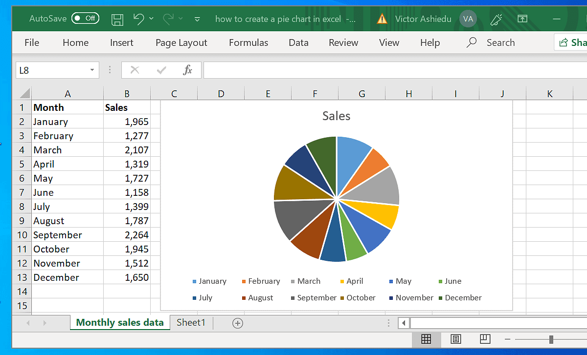
Create the data that you want to use as follows. Now select Pie of Pie from that list. To create a Pie chart in Excel you need to have your data structured as shown below.

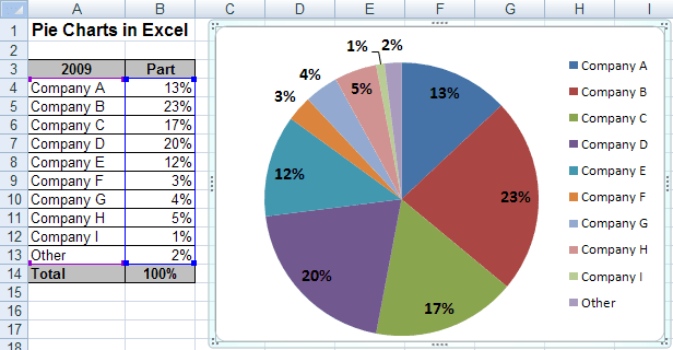
We have selected a 2D chart for instance here. Creating a pie chart in Excel is an amazing way to make all the numeric data appreciable just at a glance without the actual need to dive deep into the facts and the figures. To create a pie chart in Excel 2016 add your data set to a worksheet and highlight it.

You can now see that a 2D pie chart has been created with legends below the chart. And then click Insert Pie Pie of Pie or Bar of Pie see screenshot. The description of the pie slices should be in the left column and the data for each slice should be in the right column.

Open the document containing the data that youd like to make a pie chart with. Under the Charts section click the Pie or Doughnut Chart icon. Creating Pie of Pie Chart in Excel.

To show hide or format things like axis titles or data labels. Then click the Insert tab and click the dropdown menu next to the image of a pie chart. Creating a Pie Chart in Excel.

Go to th e Insert tab. Click on the drop-down menu of the pie chart from the list of the charts. Below is the Sales Data were taken as reference for creating Pie of Pie Chart.

In your spreadsheet select the data to use for your pie chart. And you will get the following chart. Click and drag to highlight all of the cells in the row or column with data that you want included in your pie graph.

Then select the data range in this example highlight cell A2B9. Select the range of cells containing the data cells A1B7 in our case From the Insert tab select the drop down arrow next to Insert Pie or Doughnut Chart. You should find this in the Charts group.

Follow the below steps to create a Pie of Pie chart. Click on the drop-down menu of the pie chart from the list of the charts. Select the data to go to Insert click on PIE and select 3-D pie chart.