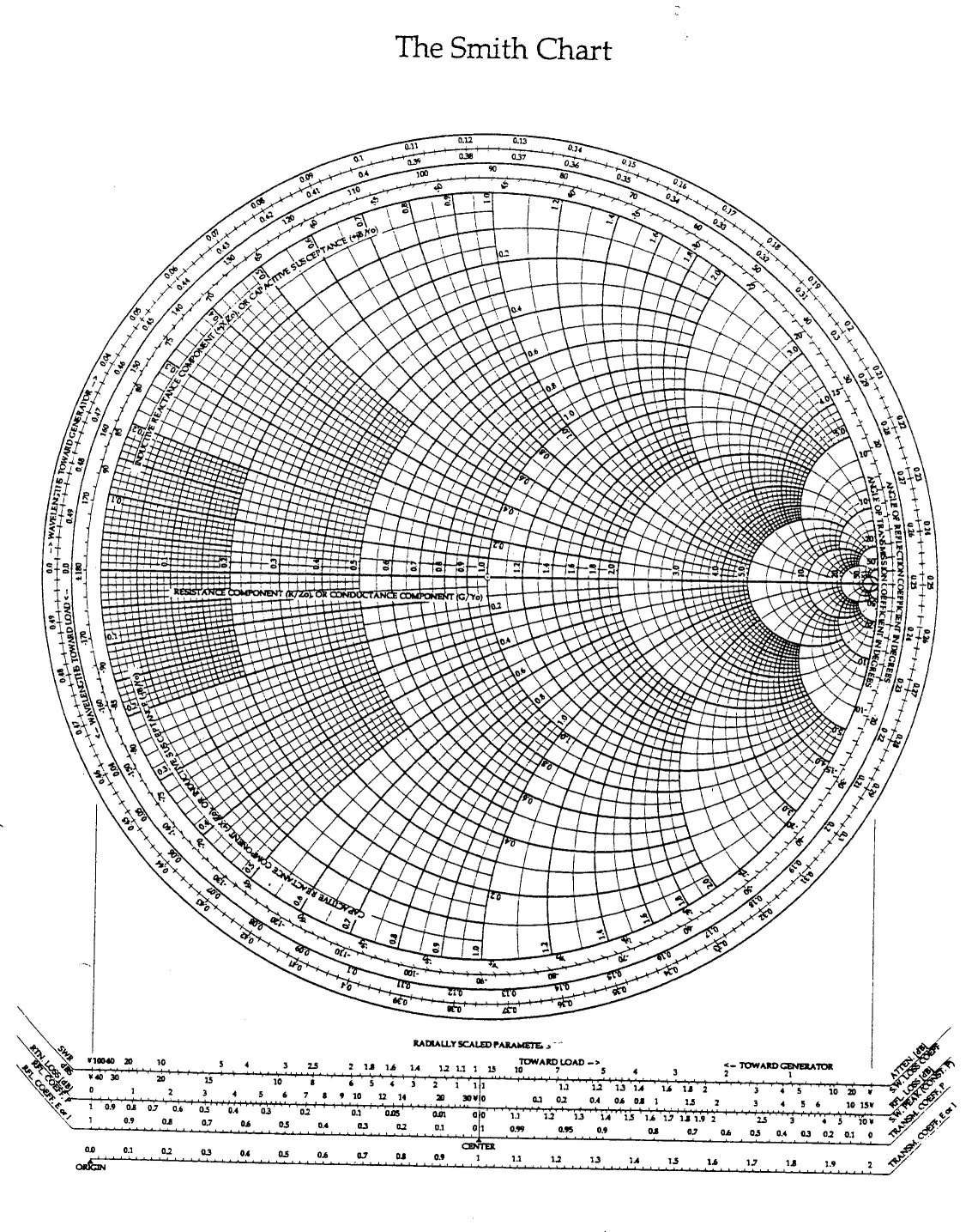
How To Use A Smith Chart


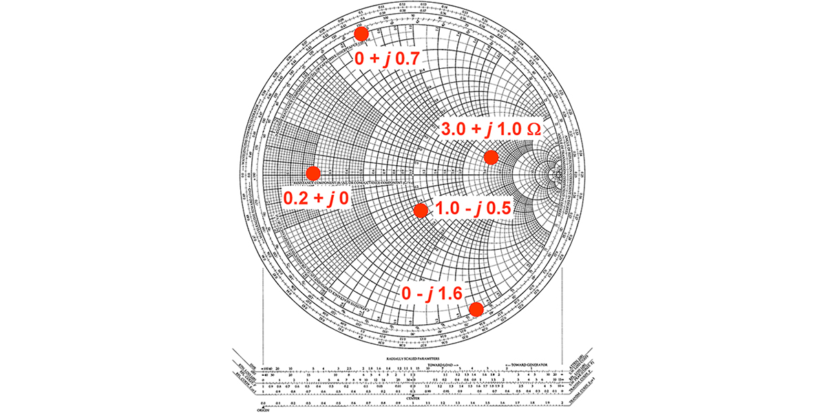
This example shows how to plot impedance data on a smithplot.
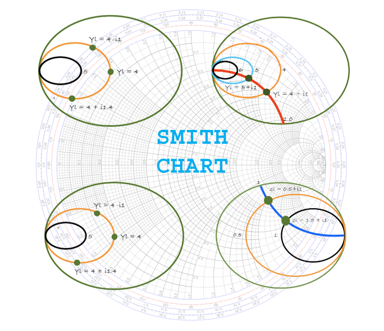
How to use a smith chart. Y 1 y 1 Y Y0 Y Y0 1Z 1Z0 1ZZ 1 0 Z Z0 Z Z0 z 1 z 1. 6 Using this transformation the result is the same chart but mirrored at the centre of the Smith chart Fig5. To start working with a Smith chart for impedance matching we need to normalize our load component that requires impedance matching to the desired system impedance.
Or it is defined mathematically as the 1-port scattering parameter s or s 11. The Moebius transform that generates the Smith chart provides also a mapping of the complex admittance plane Y 1 Z or normalized y 1 z into the same chart. The Smith chart invented by Phillip H.
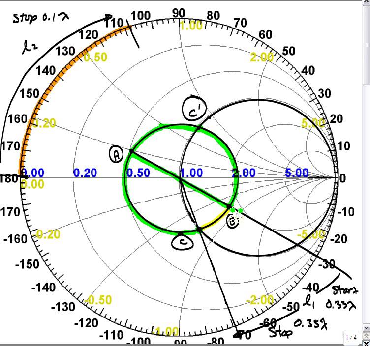
Gamma1 z2gamma z1z0. Centered at the origin draw a circle with radius of 033 then its the circle. Z1 0150 1j 0250.
The Smith Chart is a fantastic tool for visualizing the impedance of a transmission line and antenna system as a function of frequency. This introductory video describes how complex impedance and admittance are represented on the Smith Chart and how to convert between them. Plot the impedance data on the smithplot.
Locate the cross point of this r circle with coordinate and we find its 033. Reading Impedance From a Smith Chart. Smith Charts can be used to increase understanding of transmission lines and how they behave from an impedance viewpoint.
A VNA is used to. In this case it is. The Smith chart is a polar plot of the complex reflection coefficient also called gamma and symbolized by Γ.
This is really easy just divide each coordinate of. Lets verify the validity of this circle. Complex Impedance Transformations Determining VSWR RL and much more Transmission Line impedance transformations Matching Network Design.
Use a Smith Chart to design an L-section matching network to match a load Z L 25 j75 Ω to a 50 Ω transmission line at 10 GHz. Gamma2 z2gamma z2z0. Z2 0250 - 0650j.
Well call that. Based on the values of r g x and b we can roughly categorize the impedance into 4 different types. Here are links to all threeSmith Chart Basics Part 1.
Example 92 L-section matching using the Smith Chart Problem. Smith Charts are also extremely helpful for impedance matching as we will see. Since point 0330 is on this circle.
However some commercial applications and simulation tools will display impedance data in a Smith chart. The Smith chart can be used to simultaneously display multiple parameters including. Z_L 1 1.
This video is the first in a series of three videos on Smith Chart Basics. Find the r20 circle in the Smith chart. Smith and independently by Mizuhashi Tosaku is a graphical calculator or nomogram designed for electrical and electronics engineers specializing in radio frequency engineering to assist in solving problems with transmission lines and matching circuits.
We need to move. R 1 g 1 x 0 or b 0. Smith Charts can be used to increase understanding of transmission lines and how they behave from an impedance viewpoint.
1 Four types of impedance in the Smith chart. R 1 g 1 x 0 or b 0. G 1 b any value.
First we normalize z L 25 j7550 05 j15 and locate this point on the Smith Chart. Z_L by. A Smith chart is developed by examining the load where the impedance must be matched.
The system impedance might be a 50 Ohm. The Smith Chart is a highly useful tool. Convert impedance data to reflection coefficient.
Z_L into our Smith Chart coordinate system by normalizing the values. Draw that point on your Smith Chart print one out btw. The Smith Chart is used to display.
The Smith Chart is a fantastic tool for visualizing the impedance of a transmission line and antenna system as a function of frequency.