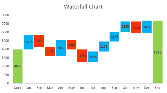
Waterfall Chart Excel 2013

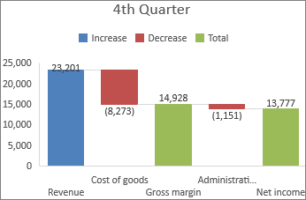
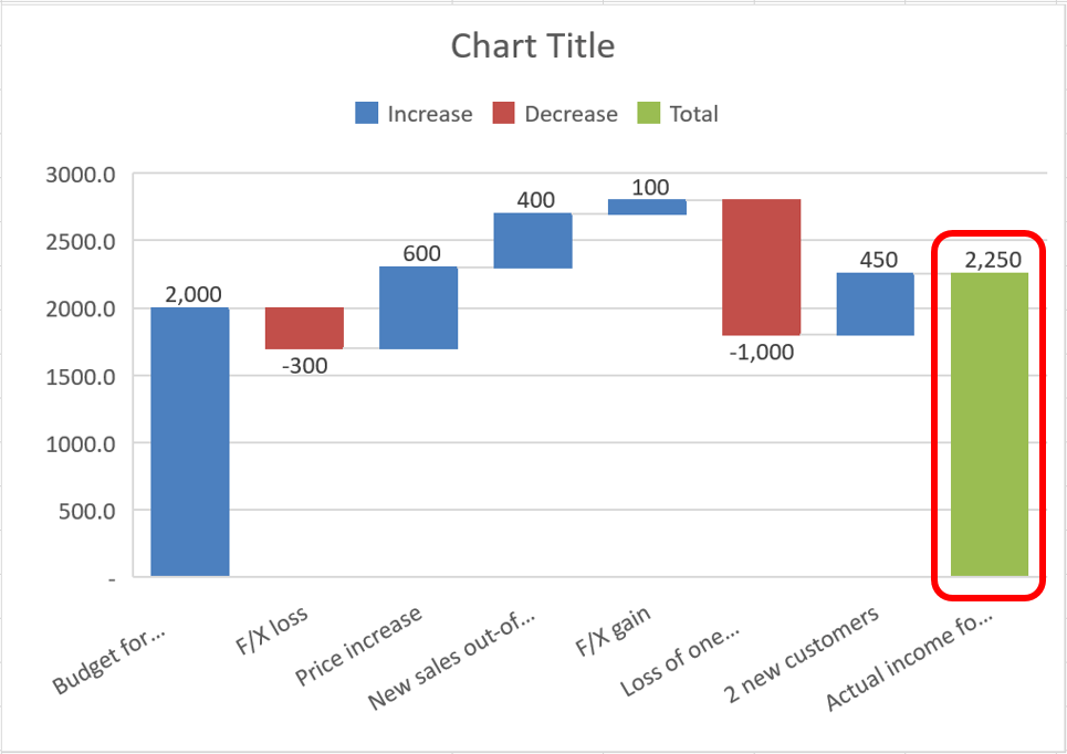
This will add labels to the subtotal and total columns.

Waterfall chart excel 2013. You just need to make the Base series invisible to get a waterfall chart from a stacked column. Layout tab Data Labels. If you have Excel 2013 and earlier versions the Excel does not support this Waterfall chart feature for you to use directly in this case you should apply the below method step by step.

To create a simple waterfall chart do the following. First you should rearrange the data range insert three columns between the original. You can make a waterfall chart within seconds and the waterfall graph will change when you change the inputs.

Excel 2007 and 2010. You can quickly format a group of data that has a starting point and an ending point and demonstrate how to get the start to the end. Excel 2016Office 365 Excel 2010-2013.

Customize a waterfall chart. Luckily we have another more collaborative way to create a waterfall chart using Smartsheet and the Microsoft Power BI. Adjust the color scheme.

Waterfall Chart In Excel 2013 And Older Datahappy. Add and position the custom data labels. Change the gap width to 20 Step 6.

Create waterfall chart in Excel 2013 and earlier versions. Build a stacked column chart. Step 2 Build the Waterfall Chart Using UpDown Bars Select cell F4 to H11 press ALT N C to insert column charts.

Now select the entire data range go to insert charts column under column chart select Stacked column as shown in the below screenshot. Adjust the vertical axis ranges. Creating waterfall charts in excel 2013.

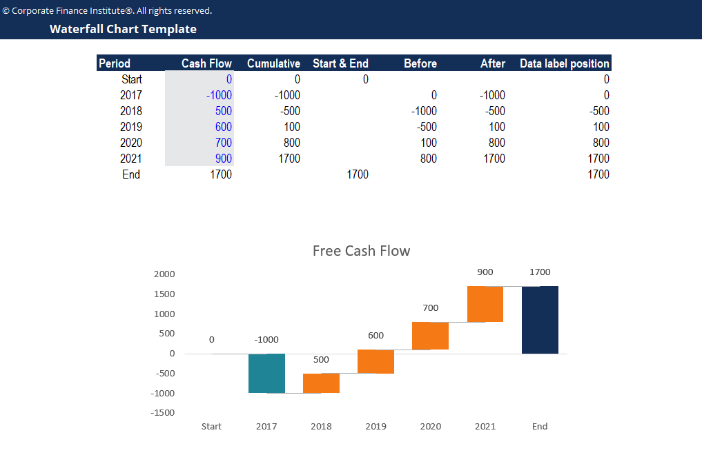
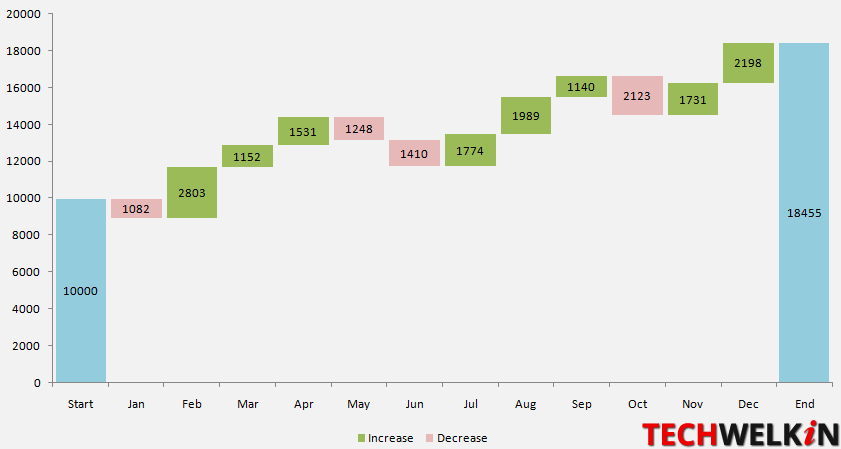
A step by step guide on How to create waterfall charts in Excel 2013 and earlier versions and in Excel 2016If you liked our Waterfall Chart in excel 201. Waterfall Chart Template Download With Instructions Supports Negative Values Excel Help Hq. Creating Waterfall Charts In Excel 2007 2010 2013 System Secrets.

Then drag up to above the column and repeat for the closing value. There you have it a simple waterfall. While a waterfall chart in Excel provides a way to visualize the change in value over a period of time it doesnt provide real-time visualization that dynamically updates as values are changed.

Add rows with empty Y data if necessary in this example 6 8 9 12 14 15 and 17 and then add two columns for. Add three columns with Y empty data Y plus data and Y minus data you can add a column for empty data and a. To create a simple waterfall chart do the following.

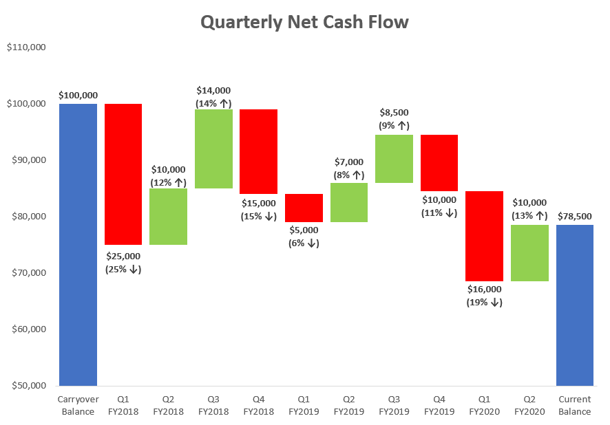
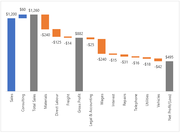
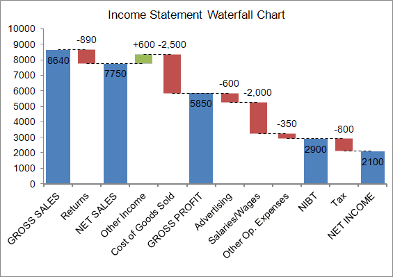
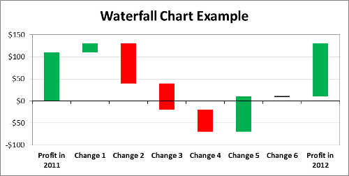
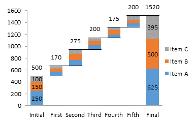
The chart demonstrates how the value increases or decreases through a series of changes. Making a waterfall chart is a powerful yet simple visually attractive and compact way of visualizing the cost structure of a business. Clean up the chart area.

In excel 2016 the chart is available by default and can be easily added through insertchartother chartswaterfall. How to Create a Waterfall Chart in Excel 2007 2010 and 2013. Click the widget button to the right of the chart Data Labels.

On your computer open a spreadsheet. Create helper columns for the original data. Select the first value twice so only it is selected.

However this is impossible to do on Excel versions 2013-2010-2007-2003 and below since the chart was only recently added in Excel 2016. In the following cells type these. Start by entering waterfall data in excel.

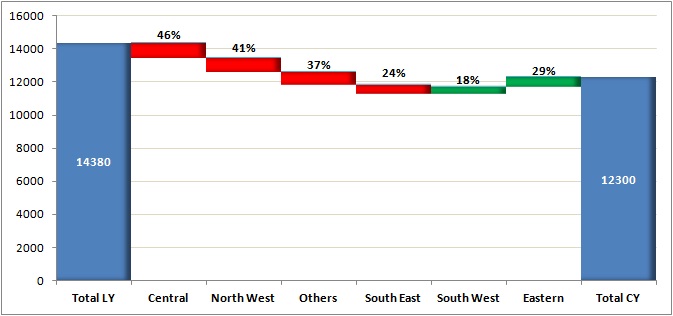
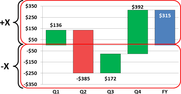
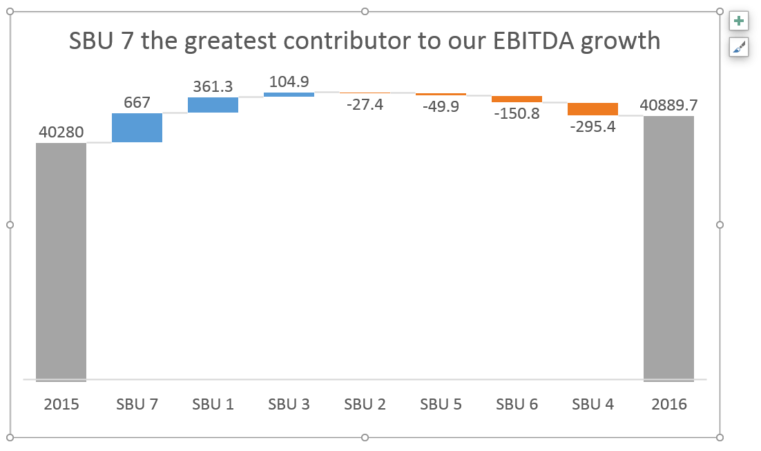
In Office 2016 this is one of the new chart templates but in Exce. Create an excel waterfall chart to show how positive and negative amounts have affected the total amount based on a starting value. How do I make a waterfall chart in Google Sheets.

This excel sheet is aimed at those pre-2016 excel users who. Hide Series Invisible Step 4. You will get the chart as below.

In 2013 CHART TOOLS à DESIGN à Add Chart Element à Data Labels à Data Callout. Waterfall Chart Templates Excel 2010 and 2013 This page demonstrates how to use a template for creating a waterfall graph that walks through changes in one variable to another. Right-click on the chart and select Change Chart Type.

Click either of the Before or After Series Lines click the green plus. The Format Data Series pane immediately appears to the right of your worksheet in Excel 2013 2016. By default the positive and negative values are color-coded.

4 Steps How To Create Waterfall Charts In Excel 2013 Data Cycle Analytics. In this video Neil Malek demonstrates how to use a template to create a waterfall chart. Creating the chart.

Create an excel waterfall chart. The easiest way to assemble a waterfall chart in excel is to use a premade template. Creating Manual Excel Waterfall Charts Excel 2013 onward.

Click on the Base series to select them right-click and choose the Format Data Series option from the context menu. Now we need to convert this stack chart to a waterfall chart with the below steps. In 2013 or earlier versions of Excel the Waterfall chart type is not present.